How do you plow a city?
Using scenario analysis to make snow plowing cheaper. Turns out classical statistics still has its uses.
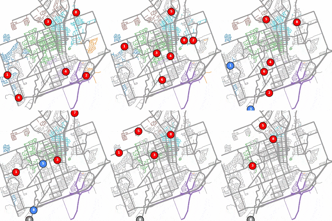
In the budgets of all snow-prone cities is an allocation for road maintenance in winter. Snow plowing, essentially. Unfortunately, plowing is as costly as it is important1, but are we always doing it the best way? One way to find out is by comparing the different variables involved in plowing (number of plows and routes, amount of snow, number of deployments) and their induced costs, which requires data.
Data
Last winter, the City of Peterborough released a tool that allows you to monitor the progress of plow operations. My first instinct on seeing the site was to simply fetch and accumulate the plow logs from the server and throw an XGBoost model at the dataset (to predict God-knows-what) when it got large enough. However, this was in May, and Spring had just come around, so there was no snow and no plows generate the data.
After searching high and low for reputable plow data and finding nothing, I turned to Mesa. It's a Python library that allows you to create spatial agents (with rules and a grid through which the agents move), which can be used for all kinds of simulation modelling. There are three basic things to know about Mesa:
- The
Agentis the core entity in every simulation. There can be many of them, each with its own internal state, and they can only act (via theirstep()method) on each timestep. - The
Modelmanages the environment theAgentsmove within, and also has its own properties. It also has astep()function which defines the unit of a timestep in the simulation. Spaceis the actual environment theAgentsmove within and it's built onNetworkx(more on that later. In my case, I only have one kind of agent, thePlowAgent, and mySpaceis the city grid, managed byCityModel.
The bulk of the logic lies in the PlowAgent's step method. When the plows are first deployed, they move to their assigned clusters in the road network2. There is a small random chance that it gets put on a random halt (my attempt at simulating traffic), and it just chills for a while if so. When the plow gets to its cluster, it checks for any roads with too much snow and adds them to its route (prioritizing arterial and collector roads over residential roads).
If the plow has a route queued up, it drives as far as its speed allows in one step3. Any road segment it crosses within its assigned cluster gets plowed (which uses salt, takes the road's snow level to zero, and logs a "plowed" event), while it just drives over any road outside its cluster without plowing4. Either way, driving burns resources, so after moving, it checks its tanks and if it's out of salt, or low enough on fuel that it might not make it back, it drops whatever route it was on, records where it was, and goes to the yard to refill.
Then repeat for the however-many plows, for the entire simulation and somehow, it works reasonably well.
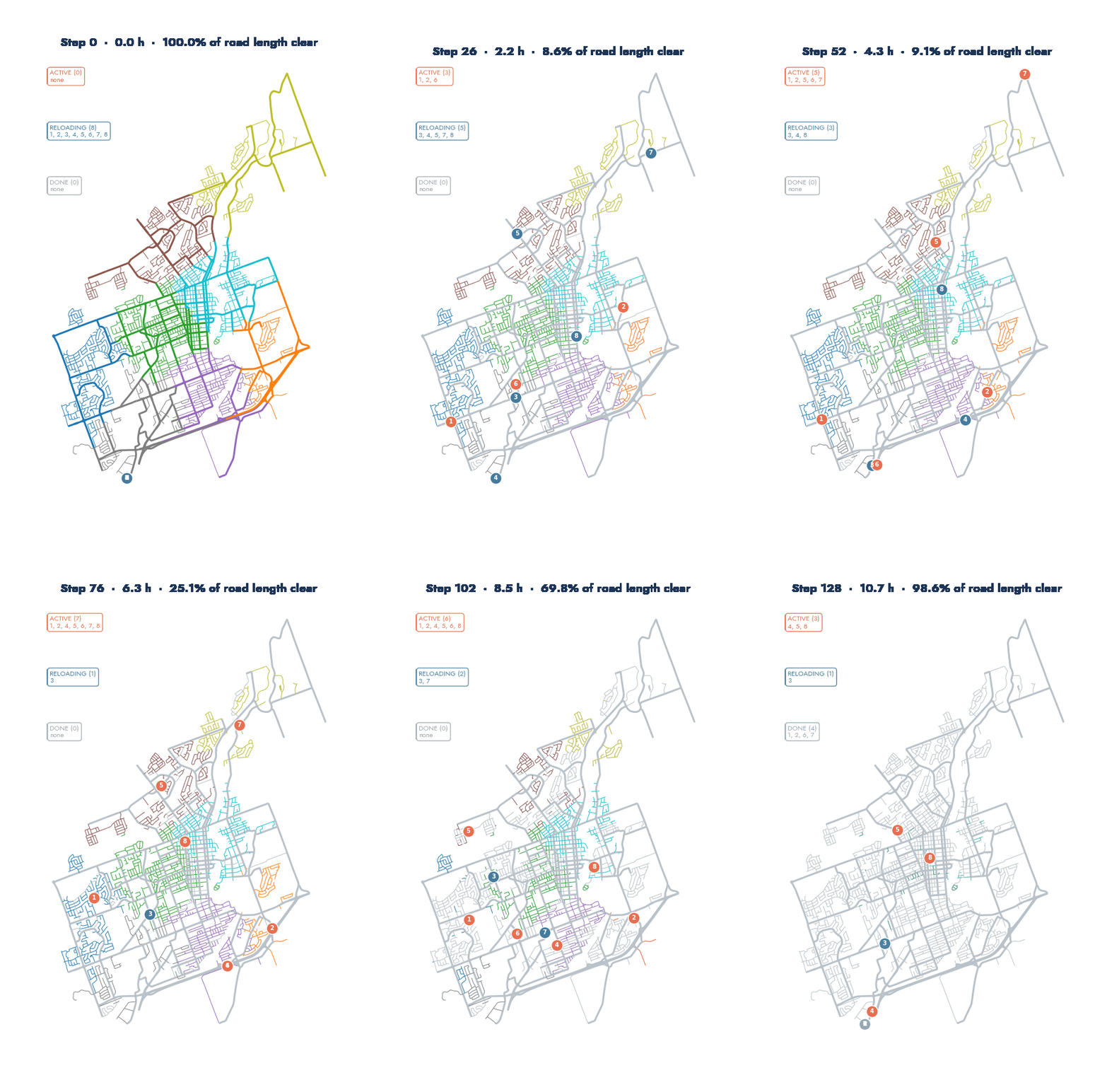
I ended up with five lists that log:
- At the plow level: Where the plow is (both ends of the road it's on), whether it's plowing, travelling, or done, how much salt and fuel it has left and, when a plow clears a road, which road, which plow, and when.
- At the network level: How much of the city network still has snow on it (below the defined threshold)5, and how much it's snowing.
- At the simulation level: What the configurations the simulation started with were, and how the sim went.
Experimentation
To experiment is to compare variations of a situation and measure their effects on a target/outcome. In my case, those are:
* Plow Duration - How long, in hours, a run takes to reach done_coverage_target
* Operation Cost (Salt, Fuel, Manpower) - cost of consumables and time
* Reach Rate - whether a run finishes before the set limit
* Coverage - % of road length below the snow depth threshold when the storm stopsThree of my outcomes are continuous, and one is categorical, and knowing my predictors (num_plows, cluster_mode, and storm_profile/historical_storms), my choice of a test6 has been narrowed. The obvious choice tests all the outcomes together, but it needs more replications than I have and can't handle a categorical outcome like Reach Rate7. Testing the outcomes separately fixes that but risks false positives from running so many tests. A permutation test avoids both of these problems.
Paired Permutation Test
A permutation test seeks to find out whether the labels we gave the configurations actually mean anything; i.e, whether the outcomes truly depend on the config or are random. It does this by shuffling (permuting) which result belongs to each config in every possible way, creating a distribution of averages for each permutation, and finding the number of averages that are as or more extreme than what we had originally (the p-value!). It is paired in this case because across each of the three configs are the same 30 storms/seeds.
Unlike MANCOVA and other parametric tests, it doesn't require a large sample size or a normal distribution. But I do have to ensure that the pairs are exchangeable and actually... paired, which they are. They use the same seed, and the simulations are performed independently.
Let's perform a test right now using three plow configs (6, 9, and 12 plows), automatic clustering, and a simulated steady storm (I'm running this using a 24x24 grid, rather than the actual Peterborough network):
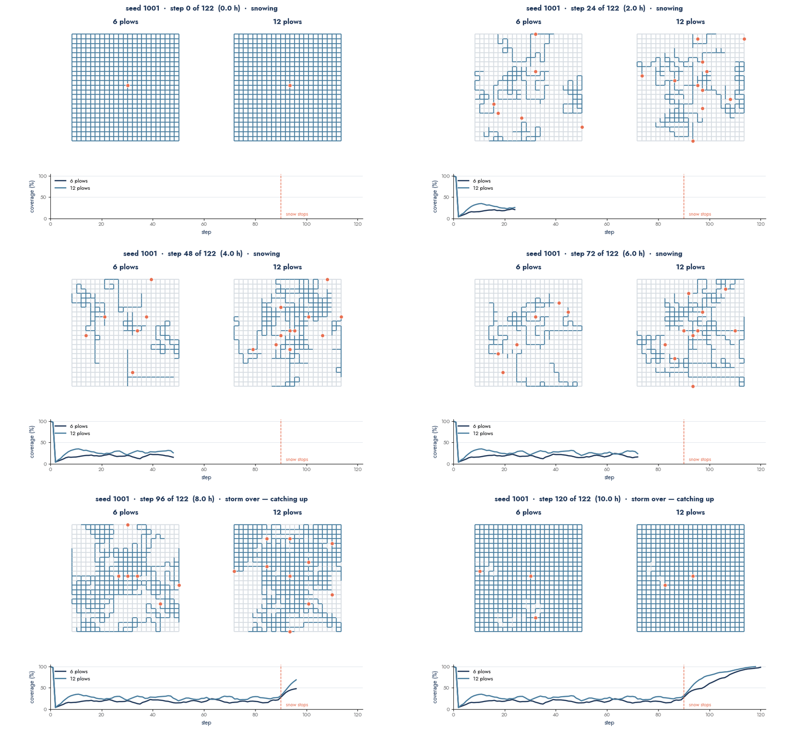
This gives me 30 matched triples, and within each, the three runs face the same storm and the same traffic & routing conditions. Consider 9 plows vs 12 plows using Plow Duration. For each seed, I subtract the 12-plow duration from the 9-plow duration (excluding runs that did not finish) and get:
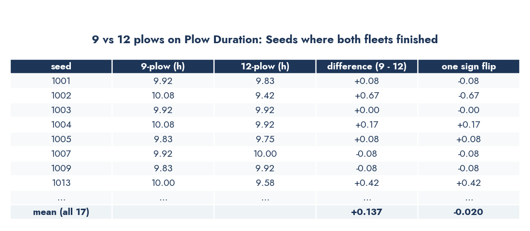
Calculating the mean of those differences and I have +0.137 hours (about 8 minutes), meaning that the smaller fleet is expectedly slower. The null hypothesis assumes that the fleet size is irrelevant to duration, and that the labels are interchangeable. So under that assumption, the signs on the differences can be reversed and nothing would change. There are (131,072) of such reversals that can be made. For each of those, I recalculate the mean difference and find out where the original mean difference of 0.137 lands.
Hypothesis?
When performing a statistical test, you want to know if there is a pattern in your data or not. The situation where there is no difference/relationship between the two scenarios you are testing, is called the Null Hypothesis ( ) in stats. Actually, the statement itself is the hypothesis. Something like: "There is no difference between the number of plows deployed and the plow duration".
The Alternative Hypothesis ( ) assumes the opposite, that there is a difference/relationship in the data. When that is the case, you reject the null hypothesis. Otherwise, you fail to reject the null hypothesis. NOT ACCEPT8. Thanks Dave :)
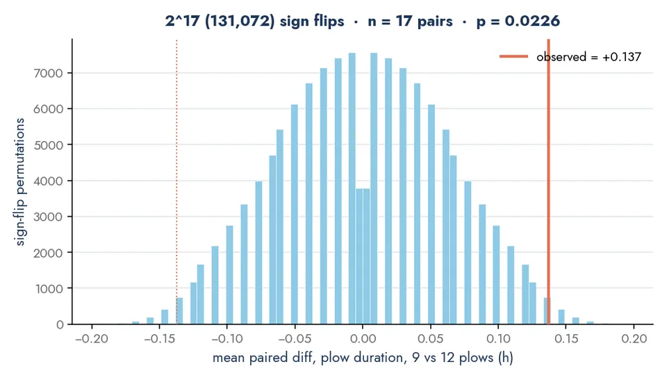
Only 2,968 out of the 131,072 permutations result in differences in duration that are as far from zero as the original difference of +0.137 hours, so the p-value is 0.023.
Remember, this p-value is the probability of seeing a gap this big (or bigger) purely by chance, if the fleet size genuinely made no difference at all. So if the value is as low as it is, it means that it's unlikely that this difference in duration is random/luck.
That test only has 17 seeds because Plow Duration is my only censored outcome9. For the outcome variables with no censoring, all the 30 seeds pair up each config, resulting in too many possible permutations for me to calculate. So I sample 10,000 of these flips10, calculate the mean difference for each of them, and then find out where the real difference lands. For example, for total cost, 6 plows vs 9 plows -$9,001 lands.
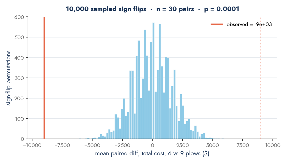
Repeating for every pair of configurations (6 vs. 9, 6 vs. 12, 9 vs. 12) and every outcome, I get a table of effects and p-values. Charting three of them:
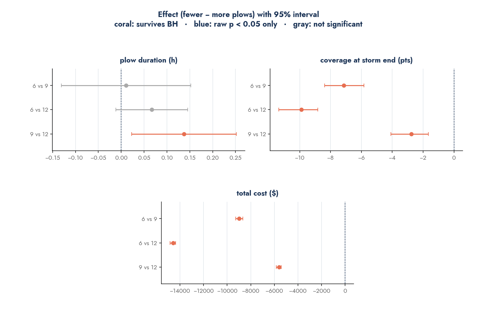
As the charts show, more plows are covering more ground by the time the storm stops and finishing more often, but they cost significantly more without actually finishing faster (for those that finish, that is).
Kaplan Meier Curves
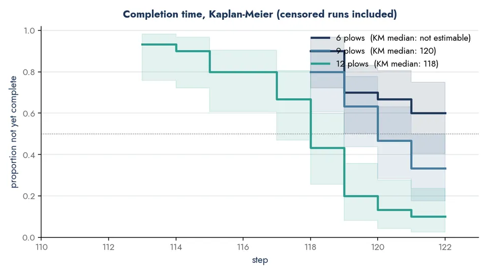
These KM curves are how I account for the runs that never finished. Averaging only the runs that did finish would inflate the weakest fleet's performance. For example, the 6-plow config's completion times look fine precisely because the 18 storms it couldn't clear have been dropped from the average. Kaplan-Meier keeps them in the picture.
Correcting for Multiple Comparisons
Using a significance level of , if the p-value falls below that, I'll assume statistical significance. But I have 21 p-values, and with my , one of them is bound to end up seeming significant by mere luck (a false positive). I can only trust each p-value if it's the only test I ran, and it isn't. I need to correct11 them somehow. Bonferroni is a choice but It'll treat the 18 tests as independent (which they aren't).
I used Benjamini-Hochberg (BH) correction which keeps the false discovery rate (FDR)12 at or below the level I pick. BH sorts the p-values by rank and keeps everything up to the last rank that meets an increasingly strict threshold:
| rank k | comparison and outcome | verdict | ||
|---|---|---|---|---|
| 1 | 6 vs 9 · coverage at storm end | <0.001 | 0.0024 | keep |
| … | (ranks 2–15: every remaining cost and coverage comparison) | <0.001 | … | keep |
| 16 | 6 vs 12 · reach rate | 0.0007 | 0.0381 | keep |
| 17 | 9 vs 12 · plow duration | 0.0226 | 0.0405 | keep (cutoff) |
| 18 | 6 vs 9 · reach rate | 0.0768 | 0.0429 | drop |
| 19 | 9 vs 12 · reach rate | 0.0923 | 0.0452 | drop |
The cut-off is the largest rank whose p-value is still under its threshold. Rank 17 in this case. Everything from rank 1 up to it stays, borderline ones included. I'm calling everything past it suggestive, because it's good to note, but might not mean much.
So what did we learn from this? More plows are, on average, more reliable, but not faster. Going from 6 to 12 more than doubles how often the fleet finishes the job and leaves the city in much better shape at the moment the snow stops. But it doesn't finish faster. The runs that completed took about the same time whatever the fleet size, and the only real duration difference was eight minutes (synthetic grid, I know). It also isn't cheap. Twelve plows cost roughly $14,600 more per storm than six.
I should note, though, that only the full 6-to-12 jump in reach rate survived the correction. The smaller differences in plow count (6 to 9 and 9 to 12) seem like real improvements but 30 replications isn't enough to prove them. I needs more seeds, and more seeds are cheap. And that's part of why I've built a pipeline around all of this.
Pipeline
By this point, I'm still in a notebook, but there are some things I'm not comfortable with.
Firstly, the experiment in this post is one of the smaller ones (a much smaller Space, one storm, one clustering mode, three plow counts) and it was still 90 full simulations. The grid is a product not a sum, so adding a second clustering mode would make it balloon to 180 sims. Each sim fills the five lists from earlier, and the plow-level ones grow fastest since they record every road a plow touches on every step. One 12-plow run generates about 11,700 rows. The 90 runs behind this post came to roughly 860,000.
Also, I don't actually look at any of these rows. The tests compare whole runs against each other, so every run has to collapse down to a single row (how long it took, how much of the city was clear when the snow stopped, what it cost).
Lastly, I want to be able to watch a run back in a browser afterwards, and specifically, pause, rewind, fast-forward.
Running the Simulations
It's a Prefect flow. Prefect is an orchestration library, which gives me retries, logging and a run history for the entire experiment workflow. It walks the full factorial grid (every combination of num_plows, cluster_mode, and the storm axis) and runs the Mesa simulation for each combination and each seed. The seed list is built once and passed to every configuration:
seed_list = [base_seed + rep for rep in range(replications)]Which seems like nothing, but the previous version gave the different plow counts different seed ranges to choose from, so two configurations never shared the same seed. My so-called "paired" comparisons were effectively comparing independent samples. Not good.
I then went ahead to cache the clusters using the resolved cluster count, rather than the configuration, since cluster_mode = None means automatic and resolves to num_plows, while an explicit number resolves to the same number for every plow count. That's three KMeans partitions for a 90-run batch, instead of 90.
Extracting
The plow data is generated by me, but some data has to be obtained externally. The road network is from OpenStreetMap, fetched via osmnx:
G = ox.graph.graph_from_place("Peterborough, Ontario, Canada", network_type="drive")It gives me every drivable road in the city, as a graph (intersections and dead ends are called nodes, road segments are called edges). I project it to UTM so distances come out in metres instead of degrees, then map the roads' tags onto the two priority tiers the plows dispatch on. motorway, trunk, primary, secondary, tertiary (and their link roads) become arterial, while residential and unclassified become residential. Then I perform the KMeans clustering on top of that.
The weather comes from Open-Meteo, for the runs using real storms. I use 15-minute snowfall rate to shape the storm, and hourly snow depth to define what's already on the ground when the run starts. Both get fetched before the grid starts rather than per run, so all runs use the same storm data.
Loading
To reduce the memory footprint, long runs checkpoint their logs periodically to parquet files as they go. At the end, the accumulated data goes to BigQuery through pandas_gbq (each table loads once per experiment). It lands in a dataset called plowcast_raw, which is the only place raw simulation output lives. Every row carries its run_id and experiment_id, which is what makes the next part possible without joining back to anything.
Currently, all this also means that the batch holds everything in memory and writes once at the end. So if a batch is at run 80/90 and fails, nothing gets written into BigQuery. Since my runs are fairly fast, I was in no rush to fix this, but this isn't ideal.
Transforming
My data is transformed using dbt and for this, I created three layers with three BigQuery datasets:
plowcast_stagingis where stuff like casting types, pinning nullable columns, and renaming happens.plowcast_intermediateholds the reusable aggregations like the road length plowed for each road, for each step, and for each cluster.plowcast_martsis what is actually used.fct_experiment_summaryis the one that the tests use. It has one row per run with the config, seed, completion step, coverage, and the resources used.
%%Or put a picture of this model in bigquery%%
The prices of my resources aren't stored here so they can be modified without having to touch the data.
This layer is also where I learned a valuable lesson. The tempting way to store snow depth is for every road, on every step, for every run, which is what I did initially. The resulting table grew with , and most of what changed in those rows was insignificant. After realizing this, I started storing events instead, and rebuilding coverage from them. So to find out the coverage at, say, step 40, I would find the last time each road was plowed, and use to predict how long it would stay clear, and check if step 40 fell outside that window.
But when snowfall wasn't constant (like when the snowstorm ends partway through plowing), it broke. The model kept on running down its timers on roads that snow stopped falling on, so a run's coverage dropped after the storm, when it should've been rising to 100%. So I stopped inferring it. The simulation already compares every road's depth against its threshold on every step, because that's how it knows when it's finished. Now, it just records the number.
Serving
Getting the runs displayed on my browser was the last challenge, and also where the marts13 came in clutch.
Previously, some charts would rebuild their history in the browser, firing up to 30 separate queries (like /street_leaderboard?as_of=03:20) just to backfill a line before it could draw it. Similarly, since a plow with no state change at a step gets no row for that step, for the plow-level chart, the browser was forward-filling from the last row at or before the playhead on every animation frame.
Both are server-side problems with a server-side answer. fct_run_timeline is one row per run per step, so the frontend fetches it once per run and indexes it by step. Thirty queries and a per-frame scan turn into one request and an array lookup. It's the only model I materialise as a table rather than a view, because it's read repeatedly while a run is being watched and its inputs only change when the run finishes.
The rest of the serving story is a small FastAPI backend sitting in front of BigQuery running parameterised queries. Where two queries are independent, it runs them concurrently rather than paying two round trips in series. If a mart is missing because dbt hasn't run, the endpoints degrade to an empty state instead of failing the whole page. And the road network is fetched once and memoised on the user's end.
With all of this, I've left the notebook. The three things that bothered me at the top are handled, and the 30 extra seeds I said I needed just cost a wider seed list and some compute time.
Footnotes
Footnotes
-
Canadian cities spend tens to hundreds of millions of dollars on snow removal alone every year. ↩
-
All routing is done using
Networkx'sshortest_path()function which uses Dijkstra's algorithm to find the ideal path between two intersections ↩ -
Speed is fixed right now regardless of snow depth. Real plows slow down in deeper snow. ↩
-
This is known as deadheading, driving without doing any actual plowing. Still burns fuel though ↩
-
Arterial and collector roads have to drop below a lower snow depth than residential streets before they count as cleared. It's same order they get prioritized in when plowing. ↩
-
A statistical test is simply a way of asking whether a pattern in your data is bigger than what pure randomness alone would produce. ↩
-
Tests like MANCOVA need enough replications to check assumptions like multivariate normality and equal covariance across groups. With 30 seeds per comparison, I can't reliably check either. ↩
-
What you are saying by failing to reject is "based on the evidence, we can't sufficiently prove x". That doesn't mean that x isn't true, but that you just can't prove it is based on what you have seen, which is the scientifically sound thing to do. ↩
-
Censoring means the outcome wasn't observed for some runs. Here, storms that never finished don't have a "plow duration" at all, so I can't just average the ones that do. ↩
-
This kind of random sampling from a huge space of possibilities, instead of checking every single one, is called Monte Carlo. ↩
-
"Correcting" here means raising the bar for what counts as significant, to make up for the fact that running many tests makes at least one false positive more likely by chance alone. ↩
-
The expected share of my flagged results that are actually false positives. Different from the family-wise error rate, which is the chance of getting even one false positive across every test I ran. ↩
-
A mart is dbt's term for a table built specifically for a downstream consumer. In this case, whoever is asking "how much snow is on this road right now?". ↩